Divide and Conquer (DnC) Hardware Cost Modeling
This notebook provides a structured workflow for calculating ASIC cell gate count estimations for specific layer designs using actual physical synthesis points. It maps data plane attributes against an Arithmetic Cost Estimation (ACE) mathematical regression topology.
Analytical Target Function:
$$\text{MAC Area} = a \cdot (X_{\text{bits}} \cdot W_{\text{bits}}) + b \cdot Z_{\text{bits}} + c$$ Where:
$X_{\text{bits}}$: Input Bit-width
$W_{\text{bits}}$: Weight Parameter Bit-width
$Z_{\text{bits}}$: Accumulator register Bit-width
$a, b, c$: Regression parameters reflecting actual hardware implementation metrics.
Prerequisites
Ensure your Python environment contains the necessary data management and calculation toolsets:
# !pip install numpy pandas scipy matplotlib keras
import io
import numpy as np
import keras.ops.numpy as knp
import pandas as pd
import matplotlib.pyplot as plt
from scipy.optimize import curve_fit
1. Synthesis Sizing Data and Hardware Mappings
# Rule-of-thumb mapping between bits and gates in memory area estimate.
MemoryGatesPerBit = {
    "Register": 10.0,
    "SRAM": 1.0,
    "ROM": 0.1,
}

# Previously calculated 3D polynomial coefficients with relative MAE < 5%.
MAC_POLY3D_PARAMS = knp.array([7.70469119, 13.76199652, -92.15756665])

# Raw hardware target area measurements generated from synthesis runs
MAC24 = pd.read_csv(io.StringIO("\n283,280,286,313,325,336,356,,\n274,290,325,372,401,428,485,,\n285,325,388,510,568,614,713,,\n308,372,509,750,865,1002,1167,,\n336,427,617,1003,1151,1309,,,\n356,480,722,1165,,,,\n"), header=None)

MAC32 = pd.read_csv(io.StringIO("\n391,365,377,410,453,433,458,507,\n364,382,418,466,497,521,578,685,\n378,418,485,594,659,721,832,1035,\n408,466,596,843,1029,1151,1321,1642,\n432,521,724,1153,1363,1512,1797,,\n457,578,830,1330,1551,1782,2273,,\n"), header=None)

MAC40 = pd.read_csv(io.StringIO("\n458,457,470,500,522,527,551,605,664\n457,475,513,561,597,616,670,782,888\n470,513,579,699,766,816,928,1150,1358\n499,561,699,996,1161,1273,1499,1850,2189\n527,612,818,1275,1545,1691,2054,2516,\n549,670,927,1496,1798,2035,2490,3294,\n"), header=None)

MAC48 = pd.read_csv(io.StringIO("\n595,550,566,594,659,624,642,694,745\n551,566,607,654,727,707,763,881,984\n566,607,679,794,871,921,1017,1270,1489\n594,655,793,1097,1285,1401,1668,2101,2378\n624,711,921,1397,1816,1950,2277,2763,3301\n642,762,1015,1669,1974,2264,2718,3631,4415\n"), header=None)
2. Defining Cost Regression and Data Alignment Pipelines
def mac_gates_polynomial_3d(xyz, a, b, c):
    """Models hardware MAC area as a sum of multiplier, accumulator, and structural offsets."""
    x, y, z = xyz
    return a * x * y + b * z + c

def gen_mac_gate_model(do_plot=False):
    """Fits the polynomial coefficients based on raw data tables."""
    # Build dimension indexes matching raw matrices shapes
    abit = np.repeat(knp.array([24, 32, 40, 48]), 54)
    wbit = np.tile(np.repeat(knp.array([1, 2, 4, 8, 12, 16]), 9), 4)
    xbit = np.tile(knp.array([1, 2, 4, 8, 10, 12, 16, 24, 32]), 24)

    mac_arrs = []
    mac_arrs_index = {}
    valid_index = []
    start_pos = 0

    for mac_acc, acc_bits in zip([MAC24, MAC32, MAC40, MAC48], [24, 32, 40, 48]):
        cur_mac = mac_acc.to_numpy().reshape(-1)
        cur_valid_index = ~np.isnan(cur_mac)
        cur_valid_mac = cur_mac[cur_valid_index]

        end_pos = start_pos + len(cur_valid_mac)
        mac_arrs_index[acc_bits] = (start_pos, end_pos)
        mac_arrs += list(cur_valid_mac)
        start_pos = end_pos
        valid_index += list(cur_valid_index)

    # Strip invalid/NaN missing parameters mapping records
    xbit = xbit[valid_index]
    wbit = wbit[valid_index]
    abit = abit[valid_index]

    # Execute multidimensional optimization curve fitting
    params, covariance = curve_fit(mac_gates_polynomial_3d, (xbit, wbit, abit), mac_arrs)
    parameter_std_deviation = knp.sqrt(np.diag(covariance))

    mac_predict = mac_gates_polynomial_3d((xbit, wbit, abit), *params)
    mae_predict = knp.mean(knp.abs(mac_predict - mac_arrs)) / knp.mean(mac_arrs)

    if do_plot:
        # Render 3D tracking scattered plots
        fig = plt.figure(figsize=(10, 6))
        ax = fig.add_subplot(111, projection='3d')
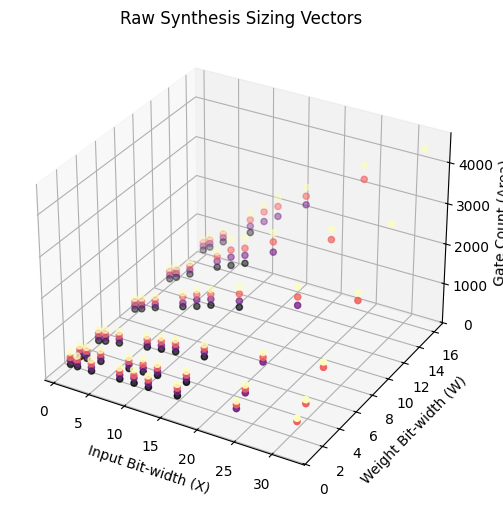
        ax.scatter(xbit, wbit, mac_arrs, c=abit, cmap='magma', label='Synthesis Data')
        ax.set_xlabel('Input Bit-width (X)')
        ax.set_ylabel('Weight Bit-width (W)')
        ax.set_zlabel('Gate Count (Area)')
        plt.title('Raw Synthesis Sizing Vectors')
        plt.show()

        # Generate surface mesh plots for distinct configurations
        x_fit = np.linspace(min(xbit), max(xbit), 30)
        w_fit = np.linspace(min(wbit), max(wbit), 30)
        xmesh, wmesh = np.meshgrid(x_fit, w_fit)

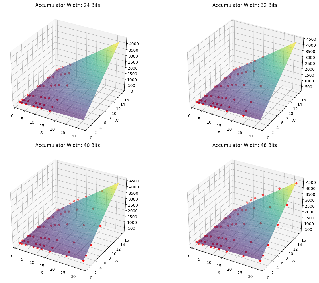
        fig = plt.figure(figsize=(14, 10))
        for idx, acc_bits in enumerate([24, 32, 40, 48], 1):
            ax = fig.add_subplot(2, 2, idx, projection='3d')
            sp, ep = mac_arrs_index[acc_bits]

            ax.scatter(xbit[sp:ep], wbit[sp:ep], mac_arrs[sp:ep], color='red', label='Data')
            amesh = np.full((30, 30), acc_bits)
            poly_fit = mac_gates_polynomial_3d((xmesh, wmesh, amesh), *params)

            ax.plot_surface(xmesh, wmesh, poly_fit, cmap='viridis', alpha=0.6)
            ax.set_title(f'Accumulator Width: {acc_bits} Bits')
            ax.set_xlabel('X')
            ax.set_ylabel('W')
        plt.tight_layout()
        plt.show()

    return params, mae_predict, parameter_std_deviation
3. Cost Evaluation Functions
def get_ace_mac_gates(xbit, wbit, abit, regen_params=False):
    """Estimates localized macro gate deployment footprints."""
    if regen_params:
        mac_params, _, _ = gen_mac_gate_model(do_plot=True)
    else:
        mac_params = MAC_POLY3D_PARAMS

    return mac_gates_polynomial_3d((xbit, wbit, abit), *mac_params)
4. Run Optimization and Predict Sizing Costs
We now trigger the calibration optimizer to determine parameters $a, b, c$, evaluate fitness errors, and test arbitrary layer structural predictions.
# Run model calibration and generate visualization plots
fitted_params, mae, std_dev = gen_mac_gate_model(do_plot=True)

print("=== OPTIMIZATION RECOVERY LOG ===")
print(f"Fitted Parameter 'a' (Mult Cost): {fitted_params[0]:.4f}")
print(f"Fitted Parameter 'b' (Accum Cost): {fitted_params[1]:.4f}")
print(f"Fitted Parameter 'c' (Base Offset): {fitted_params[2]:.4f}")
print(f"Model Mean Absolute Error (MAE):     {mae*100:.2f}%")

print("\n=== ARBITRARY HARDWARE PREDICTION TEST ===")
# Estimate gate costs for a custom hardware configuration: 4-bit inputs, 4-bit weights, 32-bit accumulator
estimated_gates = get_ace_mac_gates(xbit=4, wbit=4, abit=32, regen_params=False)
print(f"Estimated total logic gates for (X=4, W=4, Acc=32): {estimated_gates:.2f} Gates")
=== OPTIMIZATION RECOVERY LOG ===
Fitted Parameter 'a' (Mult Cost): 7.7047
Fitted Parameter 'b' (Accum Cost): 13.7620
Fitted Parameter 'c' (Base Offset): -92.1576
Model Mean Absolute Error (MAE):     4.64%

=== ARBITRARY HARDWARE PREDICTION TEST ===
Estimated total logic gates for (X=4, W=4, Acc=32): 471.50 Gates